Example

We consider the elliptic PDE with random coefficients

\[- \nabla ( a(x, \omega) \nabla u(x, \omega) ) = f(x)\]

defined on the unit square $D = [0, 1]^2$, with homogeneous boundary conditions $u(x, \cdot) = 0$ on $\partial D$.

Assume the uncertain diffusion coefficient is given as a lognormal random field $\log a(x, \omega) = z(x, \omega)$ where $z(x, \omega)$ is a Gaussian random field (see below).

• Example
• • Lognormal diffusion problems
  • Multilevel Monte Carlo
  • Multilevel Quasi-Monte Carlo
  • Multi-Index Monte Carlo
  • Unbiased estimation

Lognormal diffusion problems

First, we need to define a random field that will be used for the uncertain diffusion coefficient of the PDE. Fortunately, a Julia package that generates and samples from such random fields already exists.

using GaussianRandomFields

To specify the spatial correlation in the random field, we consider the Matérn covariance function with a given correlation length and smoothness. This function is predefined in the package.

correlation_length = 0.5
smoothness = 2.0
covariance_function = CovarianceFunction(2, Matern(correlation_length, smoothness))

We generate samples of this smooth random field using a truncated Karhunen-Loève expansion with 250 terms. To this end, we discretize the domain D into a regular grid with grid size $\Delta x = \Delta y =$ 1/128.

n = 256
pts = range(0, stop=1, length=n)
n_kl = 250
grf = GaussianRandomField(covariance_function, KarhunenLoeve(n_kl), pts, pts)

A sample of this Gaussian random field is returned by either calling the sample-function directly, or by supplying the random numbers used for sampling from the random field.

sample(grf)
sample(grf, xi = randn(n_kl))

The keyword xi corresponds to the sample $\omega$ in the defintion of the PDE.

We vizualize a sample of this random field.

using Plots
contourf(sample(grf))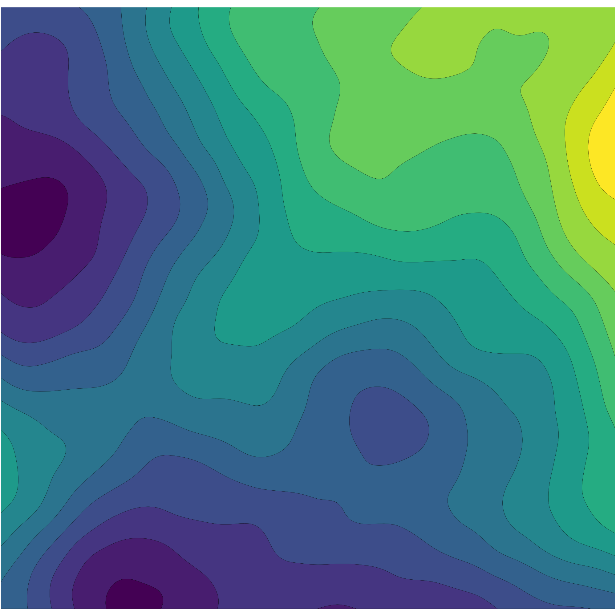

Many more options and details regarding the generation of Gaussian random fields can be found in the tutorial that accomagnies the package GaussianRandomFields.jl.

Suppose we are interested in computing the expected value of a quantity of interest derived from the solution of the PDE. For example, we might be interested in the value of the solution $u(x, ω)$ at the point $x=y=$0.5.

Multilevel Monte Carlo

The basics of any multilevel method is a hierarchy of approximations of the model problem with an increasing accuracy, but corresponding increasing cost. For the lognormal diffusion example, such a hierarchy is provided by solving the PDE on an ever finer grid. We define a hierarchy of Gaussian random field generators using

grfs = Vector{typeof(grf)}(undef, 7)
for i in 1:7
    n = 2^(i+1)
    pts = 1/n:1/n:1-1/n
    grfs[i] = GaussianRandomField(covariance_function, KarhunenLoeve(n_kl), pts, pts)
end

The corresponding system matrix that results from a finite difference discretization of the PDE with varying diffusion coefficient is returned by the elliptic2d-function from the SimpleMultigrid package.

using SimpleMultigrid
z = sample(grf)
a = exp.(z)
A = elliptic2d(a)
b = ones(size(A, 1))
u = A\b
contourf(reshape(u, n, n))

Creating an Estimator

using MultilevelEstimators

The main type provided by MultilevelEstimators is an Estimator. This type has two parametric subtypes, Estimator{<:AbstractIndexSet, <:AbstractSampleMethod}, where AbstractIndexSet is an abstract type for the index set, and AbstractSampleMethod is an abstract type for the sample method. For example, a Multilevel Monte Carlo method will have type signature Estimator{ML, MC}.

The main user interaction required by MultilevelEstimators is the definition of a sample function. This function must return a sample of the quantity of interest, and of its difference, for the given discretization parameter (or level) and random parameters. Here is an example for the lognormal diffusion problem:

function sample_lognormal(level::Level, ω::Vector{<:Real}, grf::GaussianRandomField)

    # solve on finest grid
    z  = sample(grf, xi = ω)
    af = exp.(z)
    Af = elliptic2d(af)
    bf = fill(one(eltype(Af)), size(Af, 1))
    uf = Af\bf
    Qf = uf[length(uf) ÷ 2]

    # compute difference when not on coarsest grid
    dQ = Qf
    if level != Level(0)
        ac = view(af, 2:2:size(af, 1), 2:2:size(af, 2))
        Ac = elliptic2d(ac)
        bc = fill(one(eltype(Af)), size(Ac, 1))
        uc = Ac\bc
        Qc = uc[length(uc) ÷ 2]
        dQ -= Qc
    end
    dQ, Qf
end

Thus, when the level parameter is zero, we return the value of the quantity of interest on the coarsest mesh. For a larger level parameter, we return both the difference of the quantity of interest with a coarser grid solution, and the value of the quantity of interest itself.

The sample function can only have two input parameters: a level and a vector of random parameters. For sample functions that require data (such as the precomputed Gaussian random fields in the example above), one might need to add a convenience function:

sample_lognormal(level, ω) = sample_lognormal(level, ω, grfs[level + one(level)])

Finally, for the construction of an Estimator, we also need to specify the number of random parameters and their respective distributions. For the lognormal diffusion problem, these random parameters are normally distributed.

distributions = [Normal() for i in 1:n_kl]

An estimator for the lognormal diffusion problem can thus be created using

estimator = Estimator(ML(), MC(), sample_lognormal, distributions)

Specifying options

Different options and settings can be passed on to the Estimator by supplying the appropriate keyword argument. For example, to set the number of warm up samples to 10, call

estimator = Estimator(ML(), MC(), sample_lognormal, distributions, nb_of_warm_up_samples = 10)

Running a simulation

To start a simulation for the expected value of the quantity of interest up to an absolute (root mean square) error of 5e-3, call

h = run(estimator, 5e-3)

This function will return a History object that contains usefull diagnostics about the simulation.

Vizualization of the result using Reporter

MultilevelEstimators can automatically build a set of diagnostic figures based on a History file. Load the package by

using Reporter

and generate a report by calling

report(h)

If all goes well, you should now see a webpage with diagnostic information about the simulation, similar to this one. Print-ready .tex-figures are stored locally under figures/.

Multilevel Quasi-Monte Carlo

Quasi-Monte Carlo is an alternative way to pick the samples omega. The random samples in the Monte Carlo method are replaced by deterministically well-chosen points that increase the accuracy of the estimation with respect to the number of samples. A popular type of such point sets are rank-1 lattice rules, implemented here as LatticeRule32. These points are used by default when calling the QMC-version of the Estimator

estimator = Estimator(ML(), QMC(), sample_lognormal, distributions)

Under the hood, the default lattice rule uses a 3600-dimensional generating vector from Kuo et al. It is easy to provide your own generating vector with the optional point_generator-argument.

estimator = Estimator(ML(), QMC(), sample_lognormal, point_generator = LatticeRule32("my_gen_vec.txt"))

Multi-Index Monte Carlo

It is easy to extend the lognormal diffusion example to compute multi-index differences. Instead of a difference between a fine and a coarse approximation, we now compute mixed differences.

function sample_lognormal(index::Index, ω::Vector{<:Real}, grf::GaussianRandomField)

    # solve on finest grid
    z  = sample(grf, xi = ω)
    af = exp.(z)
    Af = elliptic2d(af)
    bf = fill(one(eltype(Af)), size(Af, 1))
    uf = Af\bf
    Qf = uf[length(uf) ÷ 2]

    # compute multi-index differences
    dQ = Qf
    for (key, val) in diff(index)
        step = (index - key).I .+ 1
        ac = view(af, step[1]:step[1]:size(af, 1), step[2]:step[2]:size(af, 2))
        Ac = elliptic2d(ac)
        bc = fill(one(eltype(Af)), size(Ac, 1))
        uc = Ac\bc
        Qc = uc[length(uc) ÷ 2]
        dQ += val * Qc
    end
    dQ, Qf
end

All functionality is hidden in the call to diff(index). This function returns a Dict with as keys the indices where coarse approximations must be computed, and as values +1 or -1, specifying how these corrections must be added to the quantity of interest on the fine grid.

Multi-index sets

Different choices for the multi-index sets are available: full tensor index sets (FT), total degree index sets (TD), hyperbolic cross index sets (HC) and Zaremba cross index sets (ZC). For example, total degree (TD) index sets look like this

index_set = TD(2)
for sz = 0:5
    println("size parameter: ", sz)
    print(index_set, sz)
end

size parameter: 0
  ◼
size parameter: 1
  ◼
  ◼ ◼
size parameter: 2
  ◼
  ◼ ◼
  ◼ ◼ ◼
size parameter: 3
  ◼
  ◼ ◼
  ◼ ◼ ◼
  ◼ ◼ ◼ ◼
size parameter: 4
  ◼
  ◼ ◼
  ◼ ◼ ◼
  ◼ ◼ ◼ ◼
  ◼ ◼ ◼ ◼ ◼
size parameter: 5
  ◼
  ◼ ◼
  ◼ ◼ ◼
  ◼ ◼ ◼ ◼
  ◼ ◼ ◼ ◼ ◼
  ◼ ◼ ◼ ◼ ◼ ◼

Weighted index sets are created by specifying appropriate weiths. All weights must be smaller than or equal to 1.

index_set = ZC(1/2, 1)
for sz = 0:5
    println("size parameter: ", sz)
    print(index_set, sz)
end

size parameter: 0
  ◼
size parameter: 1
  ◼
  ◼
size parameter: 2
  ◼
  ◼ ◼
  ◼ ◼
size parameter: 3
  ◼
  ◼
  ◼ ◼
  ◼ ◼
size parameter: 4
  ◼
  ◼
  ◼ ◼
  ◼ ◼ ◼
  ◼ ◼ ◼
size parameter: 5
  ◼
  ◼
  ◼
  ◼ ◼
  ◼ ◼ ◼
  ◼ ◼ ◼

We can create an estimator the usual way:

estimator = Estimator(TD(2), MC(), sample_lognormal, distributions)

where TD(2) denotes a 2-dimensional index set.

Before running a simulation, we must precomputed the random fields on all indices.

grfs = Matrix{typeof(grf)}(undef, 7, 7)
for index in get_index_set(TD(2), 6)
    n = 2 .^(index.I .+ 2)
    pts = map(i -> range(1/i, step = 1/i, stop = 1 - 1/i), n)
    grfs[index + one(index)] = GaussianRandomField(covariance_function, KarhunenLoeve(n_kl), pts...)
end

A multi-index Monte Carlo simulation with this estimator is performed by

h = run(estimator, 5e-3)

Adaptive Multi-index Monte Carlo

Instead of using predefined (weighted or unweighted) index sets, we can also construct the index set adaptively based on some profit indicator (see [6])

\[P_\ell = \frac{E_\ell}{\sqrt{V_\ell W_\ell}}\]

where $E_\ell$ and $V_\ell$ are the expected value and variance of the multi-index difference, respectively, and $W_\ell$ is the computational cost required to computed a sample of the difference.

estimator = Estimator(AD(2), MC(), sample_lognormal, distributions)

Multi-Index Quasi Monte Carlo

Just as in standard Multilevel Monte Carlo, the Multi-Index Monte Carlo method can be extended to use quasi-random numbers instead, see [5]. The setup remains the same, just change MC() into QMC(). For example, a Hyperbolic Cross Multi-Index Quasi-Monte Carlo estimator can be created by

estimator = Estimator(HC(2), QMC(), sample_lognormal, distributions)

Unbiased estimation

The most recent development to MultilevelEstimators is the addition of unbaised multilevel estimators. In contrast to standard Multilevel Monte Carlo, a weighted sum of multilevel contributions is used, thus eliminating the bias in the estimator.

This requires a small change to the sample function, in the sense that it should now return the solutions for all levels samller than or equal to level. In the PDE example this can easily be accomplished by using Full Multigrid, see [7] and [8]. See SimpleMultigrid and NotSoSimpleMultigrid for basic example solvers. See also LognormalDiffusionProblems for a setup using Full Multigrid.

estimator = Estimator(U(1), MC(), sample_lognormal_fmg, distributions)